Appendix A. Case Examples

This appendix includes examples of statistical techniques applied to realistic groundwater data sets:

• Appendix A.1: Comparing Two Data Sets Using Two-sample Testing Methods
• Appendix A.2: Testing a Data Set for Trends Over Time
• Appendix A.3: Prediction Limits
• Appendix A.4: Using Temporal Optimization to Time Sampling Events
• Appendix A.5: Predicting Future Concentrations
• Appendix A.6: Calculating Attenuation Rates
• Appendix A.7: Comparing Attenuation Rates

A.1 Comparing Two Data Sets Using Two-sample Testing Methods

You wish to compare copper concentrations at a compliance point well with backgroundNatural or baseline groundwater quality at a site that can be characterized by upgradient, historical, or sometimes cross-gradient water quality (Unified Guidance). levels at an upgradient well at a Resource Conservation and Recovery Act (RCRA) site that has recently undergone remediation. The data sets are shown in Table A-1 below:

A.1.1 Overview

Statistical tests for comparing two groups of data are known as two-sample tests (see Section 5.11). A two-sample test is a type of hypothesis testA statistical test that determines whether one of two statements made about potential outcomes of a statistical test is true. The null and alternative hypothesis statements refer to the condition of a population parameter. The null hypothesis is favored, unless the statistical test demonstrates the greater likelihood of the alternative hypothesis (Unified Guidance). typically used to evaluate whether the meanThe arithmetic average of a sample set that estimates the middle of a statistical distribution (Unified Guidance). or medianThe 50th percentile of an ordered set of samples (Unified Guidance). concentrations of two sample populations are equal or one is greater or less than the other.

In this example, the site was contaminated in the past and now the statistical evidence is evaluated to determine if the corrective action was effective at cleaning up the site (for example, compliance well concentrations are consistent with background concentrations). Thus, the null hypothesisOne of two mutually exclusive statements about the population from which a sample is taken, and is the initial and favored statement, H₀, in hypothesis testing (Unified Guidance). is that the mean or median concentration at the compliance point is less than or equal to the mean or median concentration at the background well. The alternative hypothesis is that the compliance concentration is greater than background. The hypothesis test will be used to determine the strength of the statistical evidence that the null hypothesis is incorrect. In other words, is there statistical evidence that the compliance well concentrations are not consistent with background concentrations? Depending on the purpose of the statistical testing, a different null hypothesis may be appropriate.

There are several types of two-sample tests that can be used to compare the mean, or another population parameter of interest, of two data sets. For sites in which a small number of wells and chemicals are compared, the Unified Guidance states that the following tests may be appropriate:

Parametric Student t-tests

• Pooled variance t-test (equal varianceThe square of the standard deviation (EPA 1989); a measure of how far numbers are separated in a data set. A small variance indicates that numbers in the dataset are clustered close to the mean.)
• Welch’s t-test (unequal variance)

Nonparametric tests

• Wilcoxon rank sum test (also known as Mann-Whitney test)
• Tarone-Ware test (or Gehan's test)

The first two tests are classic parametricA statistical test that depends upon or assumes observations from a particular probability distribution or distributions (Unified Guidance). Student t-tests, while the latter two tests are nonparametricStatistical test that does not depend on knowledge of the distribution of the sampled population (Unified Guidance). and are recommended when the assumptions of the parametric tests are violated. The Tarone-Ware Test and Gehan’s Test are generalizations of the Wilcoxon rank sum test that are best for highly censored dataValues that are reported as nondetect. Values known only to be below a threshold value such as the method detection limit or analytical reporting limit (Helsel 2005). sets. It would also be possible to use prediction limitsIntervals constructed to contain the next few sample values or statistics within a known probability (Unified Guidance). to compare the two groups, but this is a more advanced approach which is not considered in this example.

A.1.2 Choose a statistical test

The most commonly used two-sample tests are Student t-tests. The pooledGroundwater samples from more than one sampling point. variance t-testA t-test, or two-sample test, is a statistical comparison between two sets of data to determine if they are statistically different at a specified level of significance (Unified Guidance). is used when the two data sets have equal variance. The Welch’s t-test is a modified version of the t-test used to compare data sets with unequal variances. You can visually compare the results of t-tests with side-by-side box plots. Since data sets will commonly have unequal variances, it may make sense to use the Welch’s t-test as it has similar powerSee "statistical power." as the pooled variance test without the requirement of equal variances.

In general, consider the use of a nonparametric two-sample test if any of the following key assumptions are violated:

• The population means are steady over time.
• Data are approximately normally distributed.
• Minimum sample size of six to eight measurements per group

The first key assumption is that the population mean is stable or steady over space and time, a property often referred to as stationarityStationarity exists when the population being sampled has a constant mean and variance across time and space (Unified Guidance).. This assumption means that a two-sample t-test cannot be performed on a data set with a trend. The Unified Guidance recommends either performing a formal trend test at the compliance well or limiting the compliance point data set to values that are representative of current conditions. The plot of the data from Table A-1 (see Figure A-1) shows a downward trend in copper concentrations at the compliance well from 2006 to present.

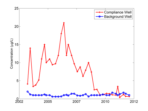
Figure A-1. Historical copper concentrations at Remediation Site A.

By visual inspection of Figure A-1, the most recent nine measurements do not have a significant trend and could be selected to represent post-remediation conditions. Since t-tests compare the mean concentrations of two data sets, using the entire compliance point data set in this case might erroneously yield the result that the compliance point concentration is greater than background.

Normality is also a key assumption of t-tests. The t-test is considered reasonably robust to this assumption, meaning that the results may still be accurate even if the normal assumption is not completely met. However, if the data set is highly skewed (coefficient of variation greater than 1.5), the test may give misleading results. For data sets that are lognormalA dataset that is not normally distributed (symmetric bell-shaped curve) but that can be transformed using a natural logarithm so that the data set can be evaluated using a normal-theory test (Unified Guidance)., the data should be first log-transformed before the t-test is applied. When the variances are equal, normality can be checked by combining the residuals for both data sets on a normal probability plot. Otherwise, check normality using graphical methods or by using a multiple group test of normality like the Shapiro-Wilk test. Normality in this example is checked for both of the data sets with histograms and normal probability plots as shown in Figure A-2.

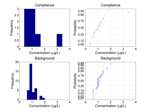
Figure A-2. Check assumption of normality.

Figure A-2 demonstrates that the data from the background well do not follow a normal distributionSymmetric distribution of data (bell-shaped curve), the most common distribution assumption in statistical analysis (Unified Guidance). and both data sets are skewed. Thus, transform the data prior to analysis or use a nonparametric method. For highly censored data sets such as the data from the background well, it can be difficult to identify a particular statistical distribution. Given the significant number of nondetectsLaboratory analytical result known only to be below the method detection limit (MDL), or reporting limit (RL); see "censored data" (Unified Guidance). in the background data set, a nonparametric method may be the best choice of statistical method for this example.

Although past guidance has recommended the use of the standard Wilcoxon rank sum test for censored data sets (assigning each group of data with the same reporting limit as a set of tied data), the current Unified Guidance cautions against this practice and recommends use of the Tarone-Ware test. The Tarone-Ware test is a generalized form of the Wilcoxon rank-sum test designed specifically for highly censored data sets. Although the test method is described in the Unified Guidance, the Tarone-Ware test is not implemented in many statistical software packages. A variant of the Tarone-Ware test that is more commonly included in statistical software is Gehan’s test.

All of the nonparametric tests discussed have similar assumptions, which include the assumption of equal variances, the assumption of a common (unknown) distribution, and temporal stability. In many cases, these assumptions will not be met completely or may be difficult to verify. Figure A-3 presents a visual comparison of the variance of the background well with the last eight measurements of data at the compliance well. This visual method is recommended by the Unified Guidance for censored data sets.

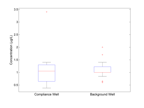
Figure A-3. Visual examination of variance.

The side-by-side box plots show that the data sets have similar buy not equal variances. It is fairly common that data from a compliance well will have a larger variance than data from a background well. From an examination of the probability plotsGraphical presentation of quantiles or z-scores plotted on the y-axis and, for example, concentration measurement in increasing magnitude plotted on the x-axis. A typical exploratory data analysis tool to identify departures from normality, outliers and skewness (Unified Guidance). in Figure A-2, it can be seen that the probability distributions are similar. From Figure A-1, neither data set has a temporal trend using only the final nine data points from the compliance well. Since there are no obvious violations of the test assumptions, perform the Wilcoxon rank sum and Gehan’s tests. Because the variances of the groups are not equal, the power of the test to detect a difference between the groups when there actually is a difference may be decreased. However, if the tests find a difference between the groups, the difference is likely to be actually present.

A.1.3 Results

The USEPA software ProUCL was used to perform both the Wilcoxon rank sum test and Gehan's test, a variant of the generalized Tarone-Ware test. A significance level of 0.05 was selected. For this example, the null hypothesis is not rejected by either of the two-sample tests, indicating there is not a significant amount of evidence that the median concentration at the compliance well is greater than the median concentration at the background well. Based on this result, the remediation of metals at Site A appears to have been successful. Technically, the test results do not show that the site has been remediated, only that there is insufficient evidence (at a 5% significance level) that it hasn’t. In other words, if more data were available, it’s possible that the conclusion would change because our hypothesis tests would have more power to detect a difference between the two data sets.

To understand how confident you should be in this conclusion, it is useful to consider the p-values and power of the tests. Using the Wilcoxon rank-sum test the null hypothesis is accepted with a p-valueIn hypothesis testing, the p-value gives an indication of the strength of the evidence against the null hypothesis, with smaller p-values indicating stronger evidence. If the p-value falls below the significance level of the test, the null hypothesis is rejected. of 0.17. Using Gehan’s variant of the generalized Wilcoxon test yields a p-value of 0.15. The p-values give an indication of the strength of the evidence against the null hypothesis (site is less than background), with smaller p-values indicating stronger evidence. Since a significance level of 0.05 is selected, consider the evidence to be significant enough to conclude that the site is greater than background if the p-value falls below 0.05. However, a p-value of approximately 0.15 could be considered weak evidence against the null hypothesis, which should be considered along with other information in order to evaluate the total weight of evidence.

Since the null hypothesis was not rejected in the example, consider the power of the test. Power is the probability that the test would detect a difference between the two groups when there actually is a difference. ProUCL can be used to calculate the required sample size for the Wilcoxon rank sum test to achieve a certain level of power at a given significance level. Specify the size of difference in concentration between the groups that should be detected, which is referred to as the width of the gray region in ProUCL. In order to achieve a power of 75% in a single-sided test, ProUCL calculates a minimum sample size of 29, given a gray region width of 2 and the default standard deviation of the test statistic of 3. Since the sample size in the example is much less than 29, the power of the test is much less than 75%. The small power of the test means that there may actually be a small statistical difference between the site and background data sets. If a small difference would have an important impact on decisions at the site, then additional data or information should be collected.

A.2 Testing a Data Set for Trends Over Time

Chlorinated solvents have historically been detected in groundwater above regulatory limits at a former dry cleaning site. Suppose you want to test whether natural attenuation is taking place and if so, whether the compliance level will be reached within a reasonable time frame without active remediation. To test this hypothesis, the vinyl chloride data show in Table A-2 from a downgradient monitoring well are analyzed for a downward trend.

Table A-2. Time Series Data

Data Set 1 (µg/L)			Data Set 2 (µg/L)			Data Set 3 (µg/L)
Date	Concentration		Date	Concentration		Date	Concentration
1/1/2000	14		1/1/2004	6		1/1/2008	10
4/1/2000	3		4/1/2004	3		4/1/2008	4
7/1/2000	10		7/1/2004	17		7/1/2008	6
10/1/2000	39		10/1/2004	30		10/1/2008	14
1/1/2001	11		1/1/2005	10		1/1/2009	8
4/1/2001	5		4/1/2005	4		4/1/2009	3
7/1/2001	19		7/1/2005	11		7/1/2009	5
10/1/2001	33		10/1/2005	31		10/1/2009	15
1/1/2002	13		1/1/2006	10		1/1/2010	9
4/1/2002	3		4/1/2006	2		4/1/2010	2
7/1/2002	10		7/1/2006	11		7/1/2010	11
10/1/2002	16		10/1/2006	12		10/1/2010	15
1/1/2003	12		1/1/2007	7		1/1/2011	6
4/1/2003	3		4/1/2007	4		4/1/2011	3
7/1/2003	11		7/1/2007	6		7/1/2011	9
10/1/2003	27		10/1/2007	26		10/1/2011	12

 

A.2.1 Overview

Various statistical tests can check the data set for a significant downward trend to demonstrate that natural attenuation is taking place. Linear regression is the most commonly used trend test, which tests the null hypothesis that the slope of the mean population is equal to zero. A one-tailed t-test is performed by comparing the test statistic to a critical point equal to the desired significance level. If the absolute value of a test statistic is larger than the critical point, then the alternate hypothesis is accepted that there is a significant downward trend at the specified significance. Alternately, a two-tailed test could be performed to test whether any trend exists. However, the use of linear regression is limited since it depends on a number of underlying assumptions that are not always satisfied in real-world environmental problems.

Alternatives to linear regression include the more robust, nonparametric Mann-Kendall and seasonal Mann-Kendall trend tests. These tests tend to perform better when analyzing real-world environmental data sets since the data do not have to conform to a particular distribution, and the tests can handle missing values and nondetects. These approaches also test the null hypothesis that there is no trend versus the alternative hypothesis that there is a trend. A Mann-Kendall statistic is formed by assigning a 1, -1, or 0 to each pair of data points depending on the sign (positive, negative, or equal) of the difference between the values. These values are then summed to form the Mann-Kendall statistic, which is compared to a critical value in a look-up table to determine if the null hypothesis is valid. When n is greater than 10, a normal approximation can be assumed based on the Central Limit TheoremStates that given a distribution with a mean, μ, and variance, σ², the sampling distribution of the mean approaches a normal distribution with a mean, μ, and a variance σ²/N as N, the sample size, increases (USEPA 2010).. In this case, a Z statistic is formed and compared to a critical point from the standard normal distribution.

As opposed to linear regression, the Mann-Kendall and seasonal Mann-Kendall tests predict the median population at any given time. This is the reason nondetects and missing values do not necessarily affect the performance of the tests. According to the Unified Guidance, nondetects can typically be replaced by half the reporting limit as long as they make up less than 10-15% of the data. In this case, be sure that a downward linear trend is not merely an artifact of lower reporting limits due to improved analytical methods. For the Mann-Kendall and seasonal Mann-Kendall tests, nondetects can comprise up to 50% of the data; as long as these values occur in the lower half of the distribution, the median will always be based on a detected result.

Section 5.7 discusses managing nondetect data in statistical analyses. In addition, Helsel (2012) provides a summary of the pitfalls of simple substitution and cautions against the method recommended in the Unified Guidance. Helsel describes three alternative approaches to deal with censored data:

• nonparametric methods after censoring at the highest reporting limit
• maximum likelihood estimation
• nonparametric survival analysis procedures

The first method is intended for use when a simple analysis is warranted. The latter methods are more powerful, but require a more advanced understanding of statistics.

The seasonal Mann-Kendall test is also especially useful because seasonal fluctuations in real-world environmental data sets may not follow a predictable pattern. If this is the case, it may not be possible to de-trend a data set before analysis with the other tests.

In this example, linear regression and the Mann-Kendall and seasonal Mann-Kendall trend tests are performed on both the seasonally adjusted and unadjusted data to evaluate whether a statistically significant trend at the α = 0.01 significance level exists. The results are then compared.

A.2.2 Visual Examination

The first step in trend analysis is to visually inspect the nature of the data set for apparent linear or cyclic trends. Cyclic trends such as seasonal patterns can mask linear trends and should be accounted for by either removing the trend from the data set prior to analysis or by using a method not affected by seasonality. More advanced statistical techniques may be required if complicated patterns are identified, such as abrupt changes in trends or impulses.

Evaluate statistical assumptions and limitations before formally testing a data set for a trend. For example, significant skewnessA measure of asymmetry of a dataset (Unified Guidance)., extreme data values, or non-normality can biasSystematic deviation between a measured (observed) or computed value and its true value. Bias is affected by faulty instrument calibration and other measurement errors, systematic errors during data collection, and sampling errors such as incomplete spatial randomization during the design of sampling programs (Unified Guidance). or invalidate linear regression results. Other assumptions inherent in linear regression depend upon the regression residuals and can only be checked after the test has been performed. Regression residuals must be normally distributed, show homoscedasticityThe equality of variance among sets of data (Unified Guidance)., and be statistically independent. Homoscedasticity means that the variance is constant over time and mean concentration.

The following figures and analysis were developed using the Matlab software package. However, many other statistical packages could be used to create similar results. The four-plot in Figure A-4 is a common visual tool that contains a time-series plot, lag plot, histogram, and normal probability plot.

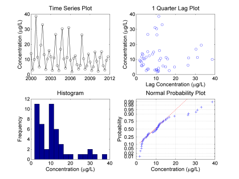
Figure A-4. Examination of original data.

The time series plotA graphic of data collected at regular time intervals, where measured values are indicated on one axis and time indicated on the other. This method is a typical exploratory data analysis technique to evaluate temporal, directional, or stationarity aspects of data (Unified Guidance). is used to check for apparent trends and outliersValues unusually discrepant from the rest of a series of observations (Unified Guidance).. Seasonal fluctuations are clearly evident in the time series plot. The lag plotA plot that displays observations for a time series against a later set of observations, or against the difference between the two sets. is used to determine whether data exhibit autocorrelationCorrelation of values of a single variable data set over successive time intervals (Unified Guidance). The degree of statistical correlation either (1) between observations when considered as a series collected over time from a fixed sampling point (temporal autocorrelation) or (2) within a collection of sampling points when considered as a function of distance between distinct locations (spatial autocorrelation).. A structure-less lag plot would indicate lack of autocorrelation in the data set. The histogram and normal probability plot are used to check for normality and skewness. The data are from a normal distribution if the histogram is symmetric and bell-shaped and the normal probability plot is linear. The data in Figure A-4 appear to be log-normally distributed and left-skewed, as is often the case with environmental data.

In order to meet the requirements of linear regression, the data set is log-transformed and the revised four-plot is shown in Figure A-5.

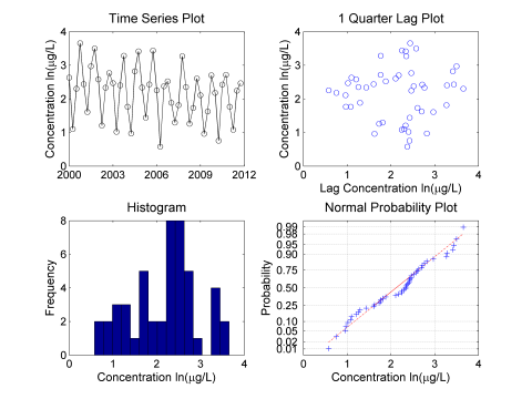
Figure A-5. Examination of log-transformed data.

The histogram is somewhat bell-shaped and the normal probability plot is close to linear, so the log-transformed data are approximately normally distributed. No skewness is now evident in the histogram and a linear trend is more evident in the time-series plot. The Lilliefors test was used to confirm that the transformed data are normal at the 5% significance level. Seasonality is also confirmed by the elliptical pattern in the lag plot.

Figure A-6 evaluates the assumptions of linear regression related to the regression residuals. The sample autocorrelation function confirms the presence of autocorrelation at lags that correspond to semi-annual and annual cycles, which violates the assumptions underlying linear regression. Sinusoidal patterns typically indicate a seasonal pattern is present. The nonparametric rank von Neumann ratio test could have also verified the assumption of statistical independence, if the data were not transformed to a normal distribution. Normality of the regression residuals is evaluated with a normal probability plot. The regression residuals appear to be approximately normal, slightly deviating from linearity. Homoscedasticity is verified by creating scatter plotsGraphical representation of multiple observations from a single point used to illustrate the relationship between two or more variables. An example would be concentrations of one chemical on the x-axis and a second chemical on the y-axis. They are a typical exploratory data analysis tool to identify linear versus nonlinear relationships between variables (Unified Guidance). of the regression residuals versus time and mean concentration. Since the scatter plots have uniform width and height and do not contain any discernible pattern it can be concluded that there is equal variance with respect to time and mean concentration.

Figure A-6. Analysis of seasonally unadjusted data.

The seasonal pattern identified in the four-plot should be accounted for by either removing the trend from the data set prior to analysis or by using a method not affected by seasonality such as the Seasonal Mann-Kendall trend test. The results of the three trend tests on the seasonally unadjusted data are shown on Figure A-7 and in Table A-3. If the absolute value of the t- or Z statistics exceeds the target then the test demonstrates that there is a downward trend. Likewise, if the calculated p-value does not exceed the target p-value (significance level), then a significant trend exists. In this example, only the Seasonal Mann-Kendall trend test is capable of detecting a downward linear trend at the 0.01 significance level among seasonal fluctuations.

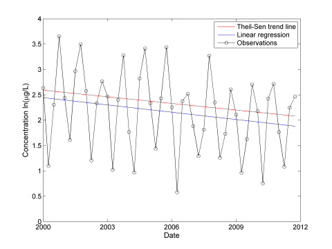
Figure A-7. Analysis of seasonally unadjusted data.

 

Table A-3. Trend test results on seasonally unadjusted data

Linear Regression Test
t-statistic		p-value		Estimated Slope (µg/L/year)
Actual	Target	Actual	Target
-1.63	2.41	0.055	0.01	-0.050
Mann-Kendall Test
Z-statistic		p-value		Estimated Slope (µg/L/year)
Actual	Target	Actual	Target
-1.70	2.33	0.045	0.01	-0.049
Seasonal Mann-Kendall Test
Z-statistic		p-value		Estimated Slope (µg/L/year)
Actual	Target	Actual	Target
-4.28	2.33	0.000009	0.01	--

 

Next, adjust the log-transformed data set to remove seasonal patterns according to the method described in Chapter 14.3.3, Unified Guidance. At least three complete, regular cycles of the seasonal pattern should be observed before adjusting the data in this manner. Figure A-8 compares the original and adjusted data sets.

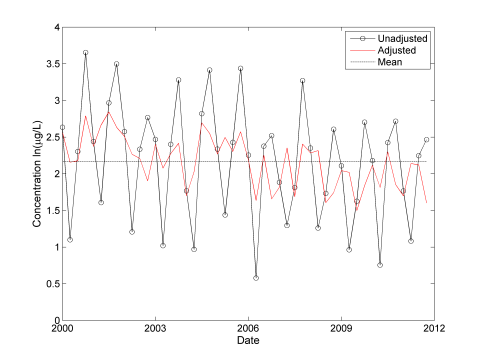
Figure A-8. Time series adjusted to account for seasonal variation.

Figure A-9 evaluates the assumptions of linear regression related to the regression residuals in the same manner as described above.

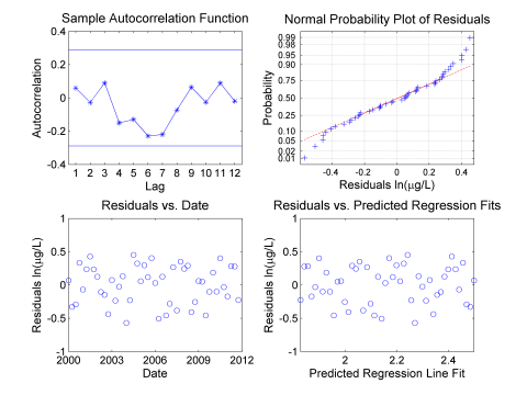
Figure A-9. Check assumptions of linear regression.

In this case, there is no significant autocorrelation identified and the normal probability plot is still only approximately linear.

Table A-4. Trend test results on seasonally adjusted data

Linear Regression Test
t-statistic		p-value		Estimated Slope (µg/L/year)
Actual	Target	Actual	Target
-5.14	2.41	0.000003	0.01	-0.059
Mann-Kendall Test
Z-statistic		p-value		Estimated Slope (µg/L/year)
Actual	Target	Actual	Target
-4.23	2.33	0.000012	0.01	-0.060
Seasonal Mann-Kendall Test
Z-statistic		p-value		Estimated Slope (µg/L/year)
Actual	Target	Actual	Target
-4.28	2.33	0.000009	0.01	--

 

All three trend tests are performed on the log-transformed and seasonally adjusted data set. The estimated trend lines and p-values are shown on Figure A-10 and in Table A-4. Once the seasonality is removed, both the regular Mann-Kendall test and linear regression also detect a significant downward trend in the data. This is evidenced by p-values lower than the target p-value (significance level).

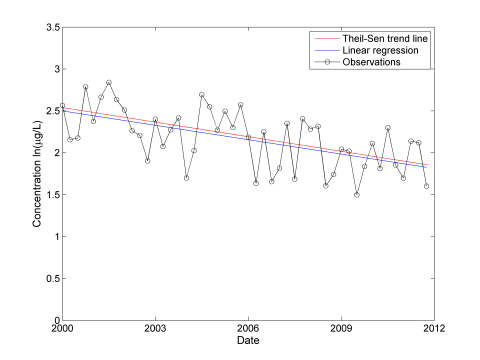
Figure A-10. Time series plot overlaid with linear regression and Theil-Sen trend line.

Once a significant decreasing trend has been identified, the estimated slope from the linear regression can be used to predict how long it will take to reach the compliance level (see Figure A-11). According to the Unified Guidance, the upper confidence limit on the mean is used to test for compliance in this situation. The confidence band is calculated according to the Unified Guidance for estimating confidence limits around a linear regression with an identified significant trend. However, the confidence band becomes quite large as the data set is extrapolated into the future so the estimated regression line is used predict that vinyl chloride concentrations will reach the federal maximum contaminant level (MCL) of 2 µg/L shortly after 2040. Site-specific information, along with the regulatory context, and input from stakeholders would be needed to determine whether this time frame is acceptable or if active remediation is warranted.

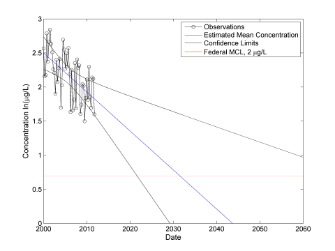
Figure A-11. How long until the compliance goal is met?

An alternative approach to assessing the progress of monitored natural attenuation was developed by the USEPA for use at CERCLAComprehensive Environmental Response, Compensation, and Liability Act sites during the five-year review process (USEPA 2011b). This approach uses the calculation of an interim remedial goal at the end of each review cycle that indicates whether natural attenuation is proceeding adequately based on a first order decay rate law. This method could be applied to any situation by using a review period of any length.

A.3 Calculating Prediction Limits

Prediction limits apply to groundwater statistics in general, but are most commonly used to understand background concentrations. Comparisons to the prediction limit provide an answer to Study Question 2, Are concentrations greater than background concentrations?

There are four categories of prediction limits:

• prediction limits for m future values
• prediction limits for future means
• nonparametric prediction limits for m future values
• nonparametric prediction limits for a future median

This example considers the first category and was taken from Example 18-1, Unified Guidance. Table A-5 presents some data for an intrawellComparison of measurements over time at one monitoring well (Unified Guidance). comparison.

Table A-5. Intrawell comparison data

Period	Date	Result (µg/L)
Background	1/1/2001	12.6*
	4/1/2001	30.8
	7/1/2001	52
	10/1/2001	28.1
	1/1/2002	33.3
	4/1/2002	44
	7/1/2002	3*
	10/1/2002	12.8
	1/1/2003	58.1
	4/1/2003	12.6*
	7/1/2003	17.6
	10/1/2003	25.3
Compliance	1/1/2004	48
	4/1/2004	30.3
	7/1/2004	42.5
	10/1/2004	15

*These values were also evaluated as nondetects in the supplemental analyses.

The 12 measurements taken during the background period are used to construct the upper prediction limit for the compliance period of four measurements. Construct and compare the upper prediction limit as follows:

1. Check the sample data for normality. For example, the Shapiro-Wilk test provides a test statistic equal to 0.947. Based on alpha=0.05 there is insufficient evidence to reject the assumption of normality. The diagnostic plots provided in Figure A-12 provide graphical information to support this conclusion.
2. Calculate the sample mean (27.52) and standard deviation (17.10).

3. Calculate the upper prediction limit based on the t-statistic. Suppose the overall confidence limit is 95% (1-alpha [0.05]). In this case there are four future measurements and the quantile for the t-statistic should be set to 0.9875 (1-0.05/4) based on assuming independence of these samples and making a simple Bonferroni adjustment. Note that Gibbons et al. 2009 warn that such simple Bonferroni adjustments do not account for the fact that the comparisons are correlated because all four compliance samples are compared to the same background.

   Calculate the upper prediction limit (73.67) as follows:

   

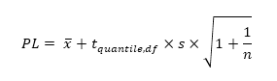
   where:

   x̄ = sample mean

   s = standard deviation

   n = number of values

   t_quantile,df = look-up value based on the t-distribution

   df = degrees of freedom (df = n-1) = 11

4. Compare the four compliance samples to the upper prediction limit. Since none of the four measurements are greater than the prediction limit, there is no evidence for an increase in concentration for this well.

Supplemental Analyses. Nondetects are a common issue for groundwater sample results. Table A-5 includes three sample results from the background period as nondetect values. This change illustrates the impacts of nondetects on background statistics. The upper prediction limit (UPL) calculations were made using ProUCL for these supplemental analyses.

• For the 95% UPL for Next 4 Observations, with three nondetects and assuming a normal distribution, ProUCL returned a value of 77.71 using the maximum likelihood estimation (MLE) method.
• For comparison, ProUCL returned a nonparametric 95% UPL for Next 4 Observations, also based on three nondetects, of 69.68 using the Kaplan-Meier method
• For the 95% UPL for Next 4 Observations, using the original background data (all detects), and assuming a normal distribution, ProUCL returned a value of 73.67 (the same value as calculated above)
• For comparison ProUCL returned a nonparametric 95% UPL for Next 4 Observations, also based on the original background data (all detects), of 58.1, which was the maximum concentration reported

With the exception of the nonparametric UPLupper prediction limit, the prediction limits calculated based on this example data set are fairly similar. This result is unusual, and for this example data set the gammaA gamma distribution or data set. A parametric unimodal distribution model commonly applied to groundwater data where the data set is left skewed and tied to zero. Very similar to Weibull and lognormal distributions; differences are in their tail behavior, and the gamma density has the second longest tail where its coefficient of variation is less than 1 (Unified Guidance; Gilbert 1987; Silva and Lisboa 2007). or lognormal based UPLs are several times larger than those calculated based on the normal distribution. Methods to evaluate nondetects in environmental data are an active area of statistical research and some of these tools are now readily available with statistical software like ProUCL. In contrast to the logic that USEPA has defined for calculating upper confidence limits (UCLs) based on varying levels of censoring and sample size there is no such guidance for UPLs or UTLsupper tolerance limits. However, it is good practice to select normal, gamma, lognormal, nonparametric UPL/UTL in that order assuming that these statistical distributions are not rejected. It is also recommended that you plot the data and the resulting UPL/UTL. Lastly reviewing the UPL/UTL calculating with various methods can help you understand how sensitive the statistic is relative to distributional assumptions.

Figures A-12 and A-13 display the results of the supplemental analyses.

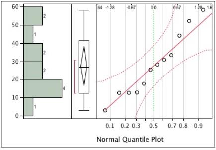
Figure A-12. Distribution diagnostic plots for background concentration data.

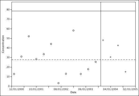
Figure A-13. Time series plot of background and compliance period data. Solid line is the upper prediction limit (73.67) and dashed line is the background period mean (27.52).

 

A.4 Using Temporal Optimization to Time Sampling Events

In this example, temporal optimization is used to examine the temporal spacing between sampling events. Groundwater sampling is often conducted on a default sampling schedule that may be monthly, quarterly, or semi-annually. In some cases, it may be possible to collect samples less frequently, but still be able to characterize contaminant concentrations over time. One statistical approach to this is iterative thinning.

Visual Sampling Plan (VSP) is an easy to use software package that can conduct this analysis. For this example, VSP was used to examine only two wells at a hypothetical site. More typically, there would be many wells at a site, and each of them would be analyzed using iterative thinning.

Figures A-14 and A-15 show the resulting plots from VSP. The original data are plotted using black dots, the smoothed data are shown with red dots, and the 90% confidence intervals are shown as blue lines. The important results is the overall trend in the data represented by the smoothed data. There is less variability in the concentrations from MW-1 (Figure A-14), so the confidence intervalStatistical interval designed to bound the true value of a population parameter such as the mean or an upper percentile (Unified Guidance). is much narrower for MW-1 as compared to MW-2 (Figure A-15). The iterative thinning algorithm identifies the frequency of sampling that would be required to reproduce the temporal trend.

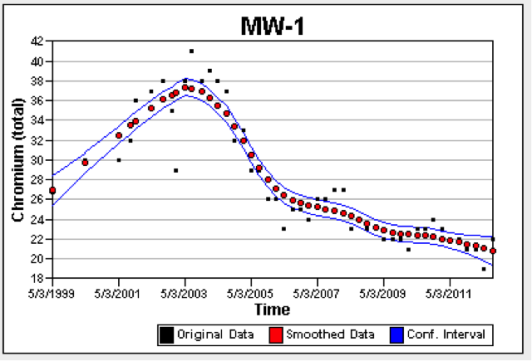
Figure A-14. VSP results for concentration (mg/l) from MW-1.

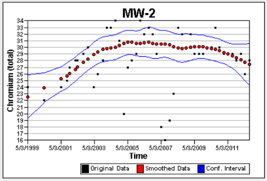
Figure A-15. VSP results for concentration (mg/l) from MW-1.

Both MW-1 and MW-2 were originally sampled quarterly. According to the VSP output, the optimal sampling frequency for MW-1 would be 202 days and for MW-2 would be 227 days. If a semi-annual frequency (180 days) were proposed for future sampling in both wells, there would be a 50% reduction in sampling costs with no significant difference in the ability to monitor trends in these wells.

A.5 Predicting Future Concentrations

This example presents the calculations for predicting future concentrations in a well based on an exponential (first-order) decay model.

For an exponential (first-order) attenuation rate, the predicted future concentration is:

Equation 1:

C_t = C₀e^-kt

 

where:

C_t = predicted concentration at time t

C₀ = current concentration

k = attenuation rate

t = time between now and the date for the prediction

For Well A, the attenuation rate for vinyl chloride is 0.2 yr^-1 with a 95% confidence interval of 0.1 yr^-1 to 0.3 yr^-1. The current vinyl chloride concentration is 1000 μg/L. Based on this information, in 10 years the predicted vinyl chloride concentration would be:

C_t = C₀e^-kt= 1000e^{-(0.2 x 10)} = 135 μg/L

A reasonable rangeThe difference between the largest value and smallest value in a dataset (NIST/SEMATECH 2012). for the prediction is:

1000e^{-(0.3 x 10)} to 1000e^{-(0.1 x 10)}= 50 μg/L to 368 μg/L

The predicted time required to attain the MCLmaximum contaminant level of 2 μg/L for vinyl chloride is 31 years.

t= Ln(C₀/C_t)/-k = Ln(2/1000)/-0.2) = 31 years

A reasonable range for the prediction is 21 years to 62 years:

t= Ln(C₀/C_t)/-k = n(2/1000)/-0.3 to Ln(2/1000)/-0.1) = 21 to 62 years

Equation 1 can be re-arranged to predict the time required to attain a specified criterionGeneral term used in this document to identify a groundwater concentration that is relevant to a project; used instead of designations such as Groundwater Protection Standard, clean-up standard, or clean-up level.:

Equation 2:

t = Ln (C₀/C_t)/-k

 

where:

t = predicted time between now and attainment of the criterion

C_t = criterion

C₀ = current concentration

k = attenuation rate

For either equation, an estimate can be obtained by using attenuation rate determined in accordance with the procedures described in Example A.6.  A reasonable range for the prediction can be evaluated using the confidence interval for the attenuation rate.

A.6 Calculating Attenuation Rates

A best estimate of the first-order attenuation rate can be obtained by fitting a first-order decay model (C_t=C₀e^-kt) to the concentration versus time data or by fitting a linear model for natural log concentration versus time data (ln(C_t) = ln(C₀)-kt). As illustrated in Figure A-16, when using the same data set, these two approaches yield identical results. In both cases, k is the first-order attenuation rate with units of time^-1. With the use of a bootstrapping method, many software packages also provide a 95% confidence band for the attenuation rate as described in Section 5.5 and Chapter 21.3.1, Unified Guidance. This confidence band is useful for evaluating the uncertainty associated with the estimated attenuation rate.

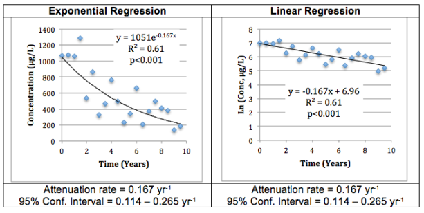
Figure A-16. Example of Regression Analysis for Temporal Trend Analysis.

.

A.7 Comparing Attenuation Rates

Two examples are presented here to illustrate the comparison of attenuation rates in two different wells at a site:

• Example 1, Different Attenuation Rates: The attenuation rate for Well A is 0.1 yr^-1 with a 95% confidence band of 0.02 yr^-1 to 0.18 yr^-1. The attenuation rate for Well B is 0.4 yr^-1 with a 95% confidence band of 0.25 yr^-1 to 0.55 yr^-1. It is reasonable to conclude that the attenuation rates in Wells A and B are different because the confidence bands do not overlap (that is the upper confidence limit for Well A (0.18 yr^-1) is smaller than the lower confidence limit for Well B (0.25 yr^-1).
• Example 2, Similar Attenuation Rates: The attenuation rate for Well A is 0.1 yr^-1 with a 95% confidence band of 0.02 yr^-1 to 0.18 yr^-1. The attenuation rate for Well B is 0.2 yr^-1 with a 95% confidence band of 0.15 yr^-1 to 0.25 yr^-1. It is not reasonable to conclude that the attenuation rates in Wells A and B are different because the confidence bands do overlap (that is the upper confidence limit for Well A (0.18 yr^-1) is larger than the lower confidence limit for Well B (0.15 yr^-1).

A.8 References

Gibbons, R.D., D.K. Bhaumik, and S. Aryal. 2009. Statistical Methods for Groundwater Monitoring. 2nd ed, Statistics in Practice. New York: John Wiley & Sons.

Helsel, D.R. 2012. Statistics for Censored Environmental Data Using Minitab and R. Second Edition. John Wiley & Sons, Inc. Hoboken, New Jersey, USA.

United States Environmental Protection Agency (USEPA). 2011. An Approach for Evaluating the Progress of Natural Attenuation in Groundwater. US EPA/600/R-11/204. December.

USEPA. 2009. Statistical Analysis of Groundwater Data at RCRA Facilities Unified Guidance. US EPA/530/R-09-007. March.

Publication Date: December 2013